This MCP server maps your code so agents read fewer files
codebase-memory-mcp's 10x token saving came with quality falling from 0.92 to 0.83 in a 31-language test. How 120x became 10x, plus setup and re-measuring.
The “one-tenth of the tokens” claim that follows codebase-memory-mcp around comes paired with answer quality that fell from 0.92 to 0.83. The tool indexes a repository once and stores functions, classes, and call relationships as a local SQLite graph. Instead of opening files, a coding agent queries that graph over MCP (the standard protocol for attaching tools to an AI). The graph is built with syntax parsing (tree-sitter) and type resolution, with no AI model involved in reading the code, and turning a question into tool calls is left to whichever agent you use. It is MIT-licensed, and as of October 27, 2026 (UTC) GitHub shows 47,549 stars, 3,911 forks, and 627 issues and pull requests combined, with the latest release being v0.12.1 from October 16. According to the paper, the repository had about 900 stars four weeks after its first release; it is now past 47,000.
This article reads the numbers behind that popularity one by one. For each figure, it follows who measured it, with which version, and against what, and it ends with the steps for refilling the same table on your own repository.
One tool, two numbers: 120x and 10x
The project’s old README put “120x fewer tokens” in its opening lines. Five structural questions cost about 3,400 tokens through the graph and about 412,000 tokens when answered by searching and reading files one at a time. Divided out, that is 121x, and the old README also phrased it as a 99.2% reduction. The current README has taken that wording out of its opening and leads with the paper’s figures instead. It states the preprint’s result across 31 repositories, “10x fewer tokens and 2.1x fewer tool calls”, pins it as “a measurement from March 2026”, and leaves the old five-query comparison as a single line calling it “an earlier comparison”.
The two numbers are not on the same yardstick. The old README’s figure came from five structural queries; the paper’s came from a test that put 12 question types to a repository in each of 31 languages. The paper’s questions also include ones that need the source lines read verbatim and ones that need every call site found without a miss.
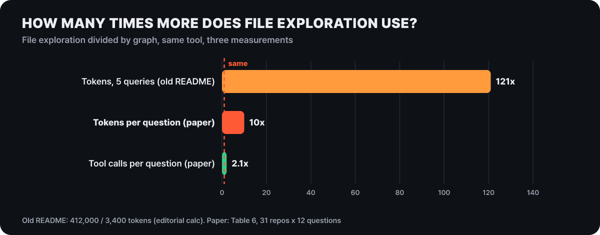 Figure 1. Three multipliers attached to the same tool. The 121x is our own division of the old README’s 412,000 and 3,400 tokens
The multiplier fell from 121x to 10x as the test widened, and tool calls come to 2.1x. What you get on your own repository depends on the mix of questions you ask. So below we open up the conditions under which the paper’s 10x was produced.
How the 10x test bench was built
The paper is arXiv 2603.27277 (submitted March 28, 2026; only v1 exists so far), and the release under evaluation is v0.5.5. At that time the tool had 14 tools and could parse 66 languages; today (v0.12.1) it has 17 tools and 162 parser grammars. For each of 31 programming languages the study picked one real open-source repository. The smallest was Terraform (HCL) with 78 nodes, and the largest was Django (Python) with 49,398 nodes. The same 12 questions went to an agent using the graph tools and to an agent exploring with file reads and grep, and both agents ran Claude Opus 4.6.
The figure below shows where each number comes from in this flow. Indexing happens once per repository, questions are asked twelve times per repository, tokens and call counts are tallied on the agent side, and the score comes from the grader at the end.
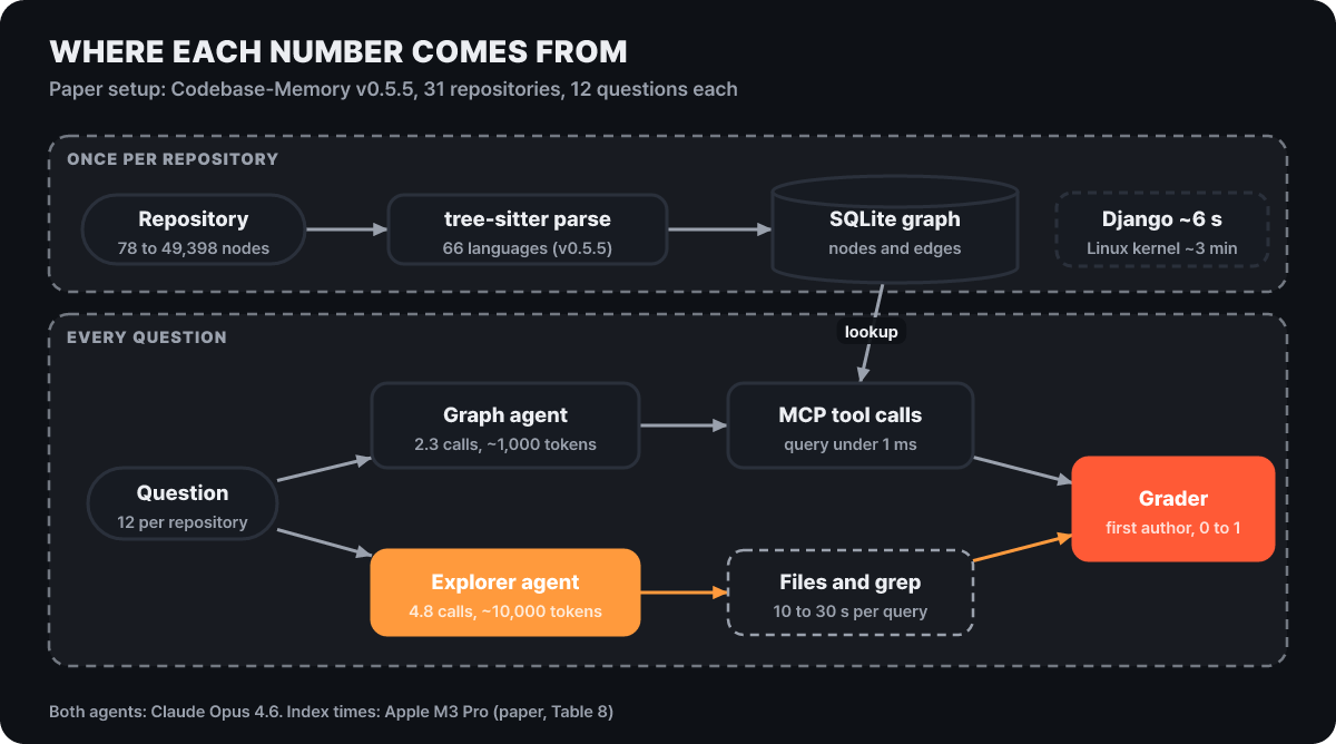 Figure 2. Structure of the paper’s test. Indexing time, query latency, token and call counts, and scores are values taken at different points
The 12 questions span nine categories, and for each category the main tool the graph side calls is fixed.
| Category (number of questions) | Main graph-side tool |
|---|---|
| Index check (1) | get_graph_schema |
| Find functions/classes (2), find by name pattern (1) | search_graph |
| Read code (1) | get_code_snippet |
| Code search (1) | search_code |
| Trace calls (2) | trace_call_path (now named trace_path) |
| Graph query (2), inheritance/implementation relations (1) | query_graph |
| File operations (1) | get_architecture |
There is something to read in this table. Five of the 12 (call tracing 2, graph query 2, inheritance/implementation 1) are structural questions and three are look-up-by-name questions, so the set includes a wide range of problems that overlap with the graph’s home turf. Scores were set against reference answers the first author made by hand, on a 0 to 1 scale: 0.80 or above passes, 0.40 to 0.79 is partial, and below 0.40 fails. The paper says it set these cutoffs “pragmatically”.
Tokens down 90%, score down 10%
The values in the paper’s Table 6 are simple. Average tokens per question are about 1,000 for the graph versus about 10,000 for file exploration, tool calls are 2.3 versus 4.8, answer quality is 0.83 versus 0.92, and one query took under 1 ms versus 10 to 30 seconds. The units are all different and hard to compare at a glance, so we redrew them with file exploration set to 100.
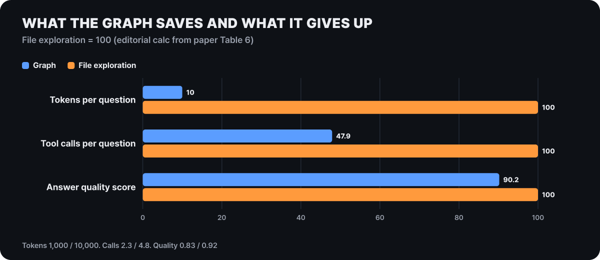 Figure 3. The editorial calculation with file exploration set to 100. The score is 0.83 divided by 0.92, which is 90.2
The lengths of the three bars show the shape of the trade. Tokens fall to 10 and calls to nearly half, while the score holds at 90.2. Converted to tokens spent per point of score, the graph side costs 1,000÷0.83≈1,205 and file exploration 10,000÷0.92≈10,870, a gap of about 9x. This is an editorial calculation dividing averages by each other.
The average of 0.83 clears the paper’s own 0.80 passing line, so on average the graph side also lands in the “pass” range. Still, inside that 0.83 there are questions that came close to full marks and questions that nearly failed. The next section looks at that distribution.
The questions where reading files directly won
The paper does not print a per-language score table. It reports, for each question type, in how many of the 31 languages each side came out ahead. On questions where the graph is the main job, such as hub detection and caller ranking, the graph tied or led in 19 of 31 languages. Conversely, on questions that need the full source context, file exploration led in 16 languages, and on grep-style questions that find every call site without a miss, it led in 10 languages.
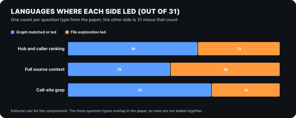 Figure 4. The paper gives one number per question type; the other side’s share is our subtraction from 31. The three types can overlap, so summing across them is meaningless
On source-context questions the graph side slips back to roughly even. The reason is that the graph deliberately does not store source lines. It stores relationships (who calls whom) but not the body of a function line by line, so a question that needs a line-level answer ends up opening the file anyway. The biggest gap came from macro-heavy C, with the graph at 0.58 against 1.00 for file exploration. Macros do not appear in the syntax tree, so the call relationships never get into the graph. In functional languages such as Haskell, OCaml, and Elixir, by contrast, the quality gap between the two approaches was about 1%.
Reading this as “C is weak” would be wrong. The project’s language benchmark document scores C as passing all 11 questions on the jq repository, and the README’s language tier table also puts C in the 90%-and-above band. The paper’s 0.58 carries the condition “a macro-heavy C repository”, and since this test pairs one repository with each language name, the value changes when the repository changes. For reference, the README’s tier table gives the pass rate of the graph tools alone: of the 35 listed languages, 17 (Lua, Kotlin, C++, Perl, Bash, and others) are at 90% or above, 16 (Python, TypeScript, Go, Rust, Java, PHP, C#, and others) are at 75 to 89%, and OCaml and Haskell are below 75%. That is a different measurement from the comparison test above.
The speed numbers come from a single M3 Pro
Every speed figure was measured on an Apple M3 Pro. Putting the paper’s and the current README’s values side by side shows which numbers for the same task survived across versions and where they changed.
| Task | Paper (v0.5.5) | README (current) |
|---|---|---|
| Full Django index | about 6 s (49K nodes, 196K edges) | about 6 s (same) |
| Full Linux kernel index (28 million lines, 75,000 files) | about 3 min (2.1M nodes, 4.9M edges) | 3 min (4.81M nodes, 7.72M edges) |
| Linux kernel fast index | none | 1 min 12 s (1.88M nodes) |
| Incremental re-index | about 1.2 s | none |
| Relationship traversal (Cypher) | under 1 ms | under 1 ms |
| Regex name search | under 10 ms | under 10 ms |
| Call path trace (depth 5) | about 0.3 ms | under 10 ms |
| Dead-code candidate detection | about 150 ms | about 150 ms |
The two “3 min” entries are times for building graphs of different sizes. For the same kernel, nodes grew from 2.1M to 4.81M and edges from 4.9M to 7.72M, so the current version puts more into the graph and still finishes in the same time. The call path trace figures of 0.3 ms and “under 10 ms” do not contradict each other either: one is a measurement and the other is an upper bound.
The most striking contrast is query latency. The paper reports graph queries at under 1 ms and the file-exploration agent at 10 to 30 seconds per question. But those 10 to 30 seconds include file reading and the model’s thinking time, so the value cannot be matched one-to-one against the graph tool itself. And these figures are what the project measured on its own computer, not a promise about yours.
The 1,000 tokens are what a repo map costs too
The “10x” is a comparison against file exploration, not against other ways of structuring code. In Table 7, the paper summarized approximate tokens per query qualitatively by method: embedding-based search (RAG) at about 2,000 to 5,000 tokens, a repo map (Aider-style) at about 1,000, a graph with an LLM attached (Neo4j and similar) at about 5,000, and this tool at about 1,000.
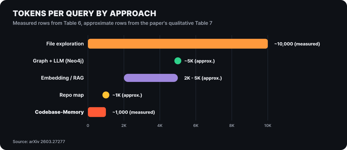 Figure 5. Two measured rows (Table 6) and three approximate rows from the paper (Table 7) on one axis. Approximate values are drawn as points or ranges
What is worth reading is that a repo map lands at the same roughly 1K. A repo map condenses key symbols and signatures and sends them to the model with each request, so it uses few tokens but cannot directly answer “who calls this function?”. In the paper’s table, the column where this tool leads is not token count but the ability to run structural queries. Because the summary a map provides and the query result a graph provides are about the same size, the selection criterion when you use them is not tokens but “will I need to ask about relationships?”
Who scored it, and the limits of the sample
The paper states its own limitations. There was only one LLM and one prompt setup in the evaluation, only one repository per language, one person (the first author) did the grading, and the pass, partial, and fail boundaries were set pragmatically. The graph holds only static structure, so calls decided at run time (dynamic dispatch, reflection) are absent. Performance figures were measured on a single piece of hardware, and there was no systematic comparison with embedding search or with other approaches such as ctags or LSP. By default query_graph returns at most 100,000 result rows.
There are limits the reader has to add as well. The first is timing. The evaluated v0.5.5 and today’s v0.12.1 differ in the number of tools (14 versus 17) and in how they parse. The v0.11.0 release notes say the tool-list response was cut by about 35%, and a change like that alters the amount that goes into the agent’s input. The second is the agent setup. The agent profiles that installation creates come in three levels: Scout (a quick provisional exploration in three or four calls), Verify (the default, checking the source directly), and Auditor (setting a scope and sweeping all of it). Which profile you run changes values like the 2.3 calls. The third is the model in use. Even with the same tool, tokens and scores split depending on how the model interprets tool results.
Setup and config files for reproducing it
The distribution channels are prebuilt binaries, npm, PyPI, Homebrew, Scoop, AUR, go install, and a Nix flake. The official quick start points to a one-line curl ... | bash, but this article does not recommend that method. A manual install is better: download the archive for your operating system and checksums.txt from the releases page, compare the hash, then unpack. The install scripts inside the archive (install.sh, install.ps1) can be opened and read before you run them, and the README explains that the scripts also verify the checksum before unpacking.
# Hash comparison example (replace the archive name with the one you downloaded)
shasum -a 256 codebase-memory-mcp-darwin-arm64.tar.gz
grep darwin-arm64 checksums.txt

# Unpack and install only the binary (leaves agent settings untouched)
tar xzf codebase-memory-mcp-darwin-arm64.tar.gz
./install.sh --skip-config
The install command (install) automatically writes MCP settings, instruction files, skills, and some hooks for the clients it detects (45 integration targets per the README). The hooks only append relevant graph information to the context when you search or read files, and do not block or change the original tool call; in Codex, you have to review and trust the installed hooks yourself in /hooks. If you do not want your home directory settings touched, install only the binary with --skip-config and register the MCP server yourself in the agent you use. To roll back, codebase-memory-mcp uninstall removes the settings, skills, hooks, and binary it wrote itself, and keeps the index files by default (--delete-indexes deletes them, --dry-run previews).
If you did not touch the settings files, register the MCP server directly. The README’s manual registration example is written into the user-scope ~/.claude.json or the project’s .mcp.json.
{
  "mcpServers": {
    "codebase-memory-mcp": {
      "command": "/path/to/codebase-memory-mcp",
      "args": []
    }
  }
}
Restart the agent, and if /mcp shows 17 tools, you are connected; say “Index this project” and indexing starts. You can also run the tools one at a time from a terminal without an agent. This CLI is used in the re-measurement below as well.
codebase-memory-mcp cli index_repository --repo-path /absolute/path
codebase-memory-mcp cli list_projects
codebase-memory-mcp cli search_graph --project my-project --name-pattern '.*Handler.*' --label Function
codebase-memory-mcp cli trace_path --project my-project --function-name Search --direction both
index_repository takes an absolute path, its response defaults to a compact tree that is easy for people to read, and adding --format json gives machine-readable JSON. Index results are stored as SQLite in ~/.cache/codebase-memory-mcp/ and survive a restart.
Supply-chain checks. Every release ships a SHA-256 checksum, a Sigstore cosign signature, and a SLSA level 3 provenance attestation from GitHub Actions, and the README explains that a release is blocked while CodeQL alerts remain. You can verify the attestation of a downloaded file yourself with gh attestation verify <file> --repo DeusData/codebase-memory-mcp. The executable is scanned with VirusTotal, the v0.11.0 release notes link the results from eight engines, and there is a note that Windows Defender may raise a false positive. The project states that it collects no statistics and that the binary sends no network requests on its own.
Settings that move the numbers for the same question
Tokens and scores shift not only with the model but also with how the graph was built. Pin the items below before you re-measure.
Index mode. The default is full, which includes semantic analysis; moderate includes semantic analysis on a filtered index; and fast is a filtered index without semantic analysis. That is why fast takes 1 minute 12 seconds on the Linux kernel. Because fast drops semantic analysis, record which mode you indexed with. Ignore rules stack in the order built-in patterns (.git, node_modules, and so on), then .gitignore, then .cbmignore, and symbolic links are always skipped.
Graph freshness. When files change, the graph has to be updated too. Watching (auto_watch) is on by default, but by default it follows only git repositories. A non-git folder stays at its last index until you run index_repository again, and turning on watch_non_git makes it watch those folders as well. If an answer looks odd, check freshness with index_status first. Automatic indexing (auto_index) is off by default, and the file-count cap is auto_index_limit.
Limits and memory. The caps on the number of files or the size indexed in one run are set with index_max_files and index_max_source_mb, and both are off by default. When a cap is exceeded, it does not produce a partially indexed graph; the whole indexing attempt fails, and the index you were using is preserved. Memory is capped with CBM_MEM_BUDGET_MB and the number of workers is set with CBM_WORKERS. For a large repository, give index_repository async: true so the daemon indexes in the background, and check progress with status: true. This is for indexing that would not finish within the time limit some IDE clients put on a single tool call.
Versions and the daemon. Releases come out fast. The release notes say that the first index after upgrading to v0.11.0 (September 15) and v0.12.1 (October 16) is a one-time full rebuild, so do not upgrade in the middle of a measurement. When you use several agents together, such as Claude Code, Codex, and OpenCode, they share one daemon per account; every active process must have the same version, the same build, and the same cache path, and if they diverge it refuses before starting any work. Logs are in ~/.cache/codebase-memory-mcp/logs.
Path restriction and shared snapshots. CBM_ALLOWED_ROOT can confine the directories index_repository may access. After resolving symbolic links and .., it rejects anything outside. With persistence: true, it writes a compressed snapshot called .codebase-memory/graph.db.zst next to the repository, and the default is off. This file is rewritten whole on each update, so committing it every time makes the repository grow sharply. The case the README cites is one team’s single file growing to about 6GB over roughly 350 commits. It is safer to set a cadence such as releases or nightly jobs, or to put .codebase-memory/ in .gitignore and let everyone index on their own.
codebase-memory-mcp config set auto_watch false       # turn off background watching during measurement
codebase-memory-mcp config set index_max_files 250000 # file-count cap (off by default)
Steps to refill the table on your own repository
The project keeps a measurement document (docs/MEASURING_SAVINGS.md) that tells you not to trust the paper’s figures as they are but to measure on your own repository. The key is not to mix three questions. Whether the answer is better, whether the graph tool is fast and stable, and whether tokens and tool calls really drop are each a different measurement. CBM’s query counter knows neither model tokens nor the agent’s total tool calls, so tokens and call counts have to be recorded by the client you use or by the evaluation harness.
- Fix the experiment. Write down the exact commit SHA of the repository, the question list and reference answers, the CBM version, index mode, and machine, and the agent's model, system prompt, and per-question budget. Use the same values for both conditions.
- Two clean worktrees. Create detached worktrees at the same SHA, one for the graph and one for file exploration, and confirm that neither has changes, including untracked files.
- Pre-check on the graph side. Right before measuring, run
index_repositoryfresh and confirm it succeeded, compare the root path and current HEAD withindex_status --verbose, then look up a symbol you verified in the source beforehand withsearch_graph. - Ask in isolated sessions. Use one session per question per condition, and keep either condition from seeing the other's answers or tool results. On the file-exploration side, allow only file listing, text search, and partial reads.
- Record per window. Write down the tokens for the answer span and for the whole session separately. If a client cannot report a window directly, leave that window out of the comparison.
- Grade the answers against the source. Score against the source at the fixed SHA, not against plausibility, and if possible keep the grader from knowing which condition an answer came from. Keep quality in a separate column next to the efficiency metrics.
A record row is one question, one condition, one window, and the format follows the one-line header below. In tool_calls, count every tool call the client made, including retries, errors, and zero-result calls, not just CBM calls.
run_id,condition,repo_sha,question_id,window,input_tokens,output_tokens,total_tokens,tool_calls,wall_time_ms,answer_artifact,quality_scoreCompare only within the same window and calculate with the four formulas below.
Token reduction (%)  = 100 × (file-exploration tokens − graph tokens) / file-exploration tokens
Call reduction (%)   = 100 × (file-exploration calls − graph calls) / file-exploration calls
Token multiplier     = file-exploration tokens / graph tokens
Call multiplier      = file-exploration calls / graph calls
If the file-exploration value is 0, do not calculate the reduction; if the graph value is 0, do not calculate the multiplier, and never plug in adjusted values. When publishing, write the raw pairs together with the number of repetitions, the aggregation method, the failed runs, the conditions you controlled, and the per-question quality scores. The document’s final principle is that a value from one repository, one question set, one model, and one machine, like the 121x or 10x above, must not be rewritten into a universal savings claim. Once this table is filled in, that value is the “multiplier” for your repository, and where it sits between the paper’s 10x and the old README’s 121x is the number that decides whether you use this tool.