llmfit rates which models run on your laptop in one go

Picture yourself at a laptop with 16GB of memory, about to download a local model to help with coding (this is a scenario made up by the editors). The list shows 7B, 14B and 32B models, and each one takes anywhere from a few minutes to an hour to download. You grab the 14B and it takes ages to produce its first sentence, or the 32B never loads at all. If every mistake costs an hour, it is better to filter by numbers before you download. llmfit, an open-source terminal tool written in Rust, does that job. It reads your hardware and turns hundreds of models into a ranking that says “with this quantization, it runs with this much headroom.” As of the check (Oct 27, 2026 UTC) it has about 38,400 GitHub stars, about 2,500 forks and an MIT license, and the latest release is v1.1.17 from Oct 8. This article follows that one laptop through installation, reading the first screen, how verdicts are calculated, where the speed numbers come from, measuring for yourself, and what-if simulation before you buy.

Why a 16GB laptop stalls in front of a model

A model card lists only the parameter count, so the guess “a 7B will surely fit in 16GB” is often wrong. Memory is spent in three places. The first is the weights, roughly parameter count × bits ÷ 8. Seven billion parameters stored at 8 bits come to about 7GB, and at 4 bits (quantization: a method that shrinks weights to fewer bits) about 3.5GB. The real bits per weight differ by method, so the file can be larger or smaller than this, but the point holds that the same model roughly doubles or halves with each quantization step. The second is the KV cache, the scratch memory the model builds up so it does not have to recompute what it has already read. It grows as the context gets longer. The third is runtime headroom and memory fragmentation.

You can gauge the size of the KV cache from the concurrent-session example in the llmfit docs. Load Qwen2.5-7B-Instruct at Q4_K_M into 24GB of memory and the weights take 5.1GB, leaving an 18.9GB KV cache budget. One session with a 4,096-token context takes 0.22GB, so the math allows up to 85 sessions at once. A longer context raises the cost per session, so fewer sessions fit in the same budget. Even if you run a single session on a laptop, the moment you paste in a long document, the same model becomes a different size.

So “does the model fit?” is not a number about one model. It is an answer you only get by putting together the model, the quantization, the context length and your memory. That calculation is exactly what llmfit does.

Install it, and turn off the dashboard first

The official README lists several ways to install. Using a package manager makes the source easier to verify.

# macOS · Linux
brew install AlexsJones/llmfit/llmfit

# Windows
winget install --exact --id AlexsJones.llmfit     # or scoop install llmfit

# Run without installing (when you have the Python tool uv)
uvx llmfit

The README also has a curl ... | sh quick install, uv tool install -U llmfit, MacPorts, a source build (cargo build --release) and a Docker image (ghcr.io/alexsjones/llmfit). With a downloaded script that runs immediately, it is better to get in the habit of opening it and reading it first.

There is one thing to know about the first run right after installing. According to the docs, when you run llmfit with no arguments outside JSON mode, a web dashboard also starts in the background on 0.0.0.0:8787. That means other computers on the same network can open it, and the screen shows your hardware details and installed models. If you use it on a café or office network, turn it off from the start.

1. Run it with llmfit --no-dashboard. If you want to keep the dashboard on, you can limit access to your own computer with the environment variable LLMFIT_DASHBOARD_HOST=127.0.0.1 (the port is LLMFIT_DASHBOARD_PORT)
2. Check that the detected CPU, RAM, GPU and backend show up at the top. If this line is wrong, every number below it is wrong
3. To see just the specs, use llmfit system, and for the raw detection output, llmfit doctor. The doctor command exists for bug reports

Separately, when you open the REST server with llmfit serve, the default address is 127.0.0.1, and you have to pass –host 0.0.0.0 explicitly to expose it outside. Just remember that the two defaults differ.

How to read the columns on the first screen

This is how llmfit reads your hardware, as laid out in the official docs.

Hardware	How it is detected	VRAM reported
NVIDIA	nvidia-smi (VRAM summed across multiple cards)	Exact dedicated VRAM
AMD	rocm-smi	Detected, but VRAM may be unknown
Intel Arc (discrete)	sysfs	Exact dedicated VRAM
Intel Arc (integrated)	lspci	Shared system memory
Apple silicon	system_profiler	Unified memory (VRAM = RAM)

If the laptop in this example is Apple silicon, memory is unified, so the full 16GB is the whole pool. Once detection finishes, the model table appears, and the columns the docs’ TUI description lists are Inst, Model, Provider, Params, Score, tok/s, Mem%, Ctx, Date, Quant, Mode, Fit and Use Case. The figure below picks only the columns directly tied to the verdict and draws an imagined laptop. The docs have no real output example, so the column names come from the docs and the numbers are assumed values the editors calculated by the verdict rules.

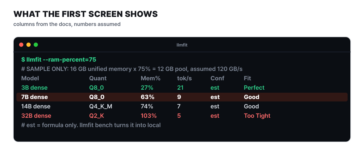Figure 1. An imagined screen with 75% of 16GB unified memory (12GB) as the pool (editors’ calculation, all numbers assumed)

The 7B row fills 63% at Q8_0, so it is Good, and the 32B, even at the smallest step, takes 103%, so it is Too Tight. The est in the Conf column marks a speed that was computed from the formula alone, and that column gets its own section later.

Score is the sum of four 0 to 100 sub-scores per model.

Item	What it looks at
Quality	Parameter count, the reputation of the model family, a penalty for quantization, fit to the use case
Speed	Tokens per second estimated from backend, parameters and quantization
Fit	Memory efficiency (the best range is 50 to 80% of available memory)
Context	Whether the model can handle the context length the use case needs

The four scores are combined with weights that depend on the use case (general, coding, reasoning, chat, multimodal, embedding). In the docs’ examples, chat puts a weight of 0.35 on speed, and reasoning puts 0.55 on quality. For the coding use case, a per-family benchmark table compiled from public leaderboards feeds the quality score, so a small model that is strong at coding can beat a large general-purpose one. Families missing from the table are estimated from the name. In the scene of hunting for a coding assistant on a laptop, setting the use-case filter to coding with the U key makes the ranking easier to read.

Cut usable memory to 75% and ask again

The default calculation counts all of the laptop’s memory as yours. But you will run the model with a browser and an editor open, so it is closer to reality to subtract the share the operating system and apps use before asking. The percent option added in v1.1.17 is for that.

llmfit --ram-percent=75 recommend --json --use-case coding --limit 3

According to the docs, --ram-percent also lowers the VRAM ceiling on unified-memory systems (it cannot be combined with --ram). 75% of 16GB, which is 12GB, becomes the new pool, and the fit verdict is decided by one number, “required memory ÷ usable memory.” Up to 60% is Perfect, up to 85% is Good, up to 98% is Marginal, and anything above is Too Tight. With a 12GB pool, Perfect goes up to 7.2GB, Good up to 10.2GB and Marginal up to about 11.8GB. Because the boundaries are ratios, the larger the pool, the larger the models that earn the same grade.

The figure below stacks, for each pool size, how many GB of required memory each of the three grades extends to. The length of one bar is 98% of the pool.

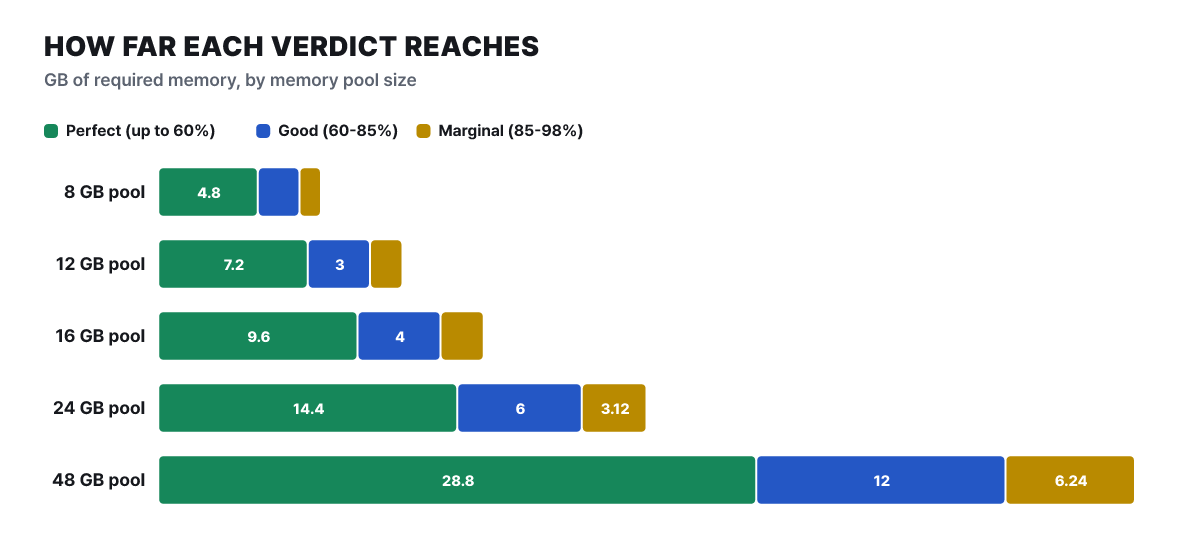Figure 2. Verdict bands by pool size (editors’ calculation, boundary ratios from the docs)

Perfect on a 12GB pool ends at 7.2GB, so a Q4-class 14B (about 9GB, assumed) stays at Good on the laptop, and you would have to drop to 7B or below to earn Perfect. The same model is Perfect on a 24GB pool.

There is a reason the line is drawn at 98%. If you fill memory to the brim, the model does not actually load because of allocation headroom and fragmentation. The docs also note a flaw in the older method. When the verdict used a recommended-RAM value set at twice the model size, a 23GB model filling 96% of a 24GB card still came out Perfect, while a 9GB model using only 56% of a 16GB card got only Good. Now the verdict uses the fill ratio alone.

The Mode column in the table also tells you that the way a model runs caps the best grade it can get.

Mode	Meaning	Best grade
GPU	The model fits in VRAM	No cap (whatever the ratio says)
MoE offloading	Active experts in VRAM, the rest in RAM	Good
CPU+GPU	VRAM falls short and spills into RAM, with only part computed on the GPU	Good
CPU	Runs from RAM with no GPU	Good

The last three modes cannot earn Perfect, which means “roomy and running on the GPU,” so Good is the ceiling. They are not pushed down to Marginal, though, because a model that fits comfortably in RAM can actually run.

The quantization is not fixed either. llmfit tries from Q8_0, the best quality, and picks the first step that fits your memory. If no step fits at the full context, it halves the context and tries again. That is why the same model in the list can show a different Quant on your computer and on a friend’s. The 32B dropping all the way to Q2_K in Figure 1 is also a result of this rule.

Press on the candidates to check the assumptions

Once the ranking is up, filtering is faster than reading from the top. The main TUI keys are these.

1. Cycle the fit filter with f (all, runnable, Perfect, Good, Marginal). For everyday use, keep only Perfect and Good
2. Filter by name, provider, parameters or use case with /, and change the sort column (score, parameters, memory ratio, context, date) with s
3. Press Enter on a model you care about to open the detail screen. This is where you check which assumptions a number rests on
4. Mark two models with m and compare them side by side with c. If you already have models downloaded, i puts the installed ones first
5. If you like one, download it with d. If more than one runtime can download it, a picker window appears. All shortcuts are under h

Gathered into a checklist, here is what to confirm before you download.

• Is Mem% below 85% (also check the assumed context length on the detail screen)
• Has the Quant stayed at Q4 or above? Going too low adds a penalty to the quality score
• If Conf next to tok/s says est, read the number only as a rough estimate
• Have you put it side by side with a model from a different family for the same use case using m and c

Mixture-of-experts models are wrong if you use the same ruler

If Mixtral or DeepSeek-family models are in the list, you should know the calculation differs. A MoE (mixture of experts) model uses only some of its expert blocks for each token, so budgeting memory by the total parameter count overestimates what it needs. llmfit recognizes these models automatically. In the docs’ example, Mixtral 8x7B has 46.7B total parameters but about 12.9B active per token, and with expert offloading the VRAM requirement drops from 23.9GB to about 6.6GB in the calculation. A model that fills 99.6% of a 24GB card and is Too Tight when assumed fully on the GPU becomes a usable candidate when only the active experts sit in VRAM and the rest in RAM. In that case, though, the Mode is MoE offloading, so the best grade is Good.

Speed is also estimated from active parameters. For models with the full architecture details (hidden size, layer count, expert intermediate size, vocabulary size), the data read per token is split into “expert weights, whose size changes with quantization” and “attention, router and embedding weights, which do not.” When information is missing, the active parameters are multiplied by a per-architecture correction value. The docs say that before this correction existed, newer architectures with 128 or more experts were modeled as far too slow, so gpt-oss-120b came out about 2.6 times too low, and such models were fixed by adding their own correction entries. Read it as a signal that the speed column can wobble more for models with newer architectures.

Where does the tok/s column come from

Token generation is assumed to be limited by memory bandwidth, so the calculation assumes the weights, the size of the model, are read once per token: (GPU memory bandwidth ÷ model size) × efficiency factor. The default efficiency factor is 0.55, a lump value covering kernel overhead, KV cache reads and memory controller effects. According to the docs, this method was verified against Apple silicon and NVIDIA T4 benchmarks posted in the llama.cpp repository. The bandwidth fed into the formula is looked up by GPU name in a table of about 80 entries (NVIDIA, AMD, Apple silicon), and if it is not in the table, it falls back to per-backend constants.

The figure below plugs four bandwidths and four model file sizes into this formula. The lower a dot sits, the slower it is, and the dotted line is 10 tokens per second.

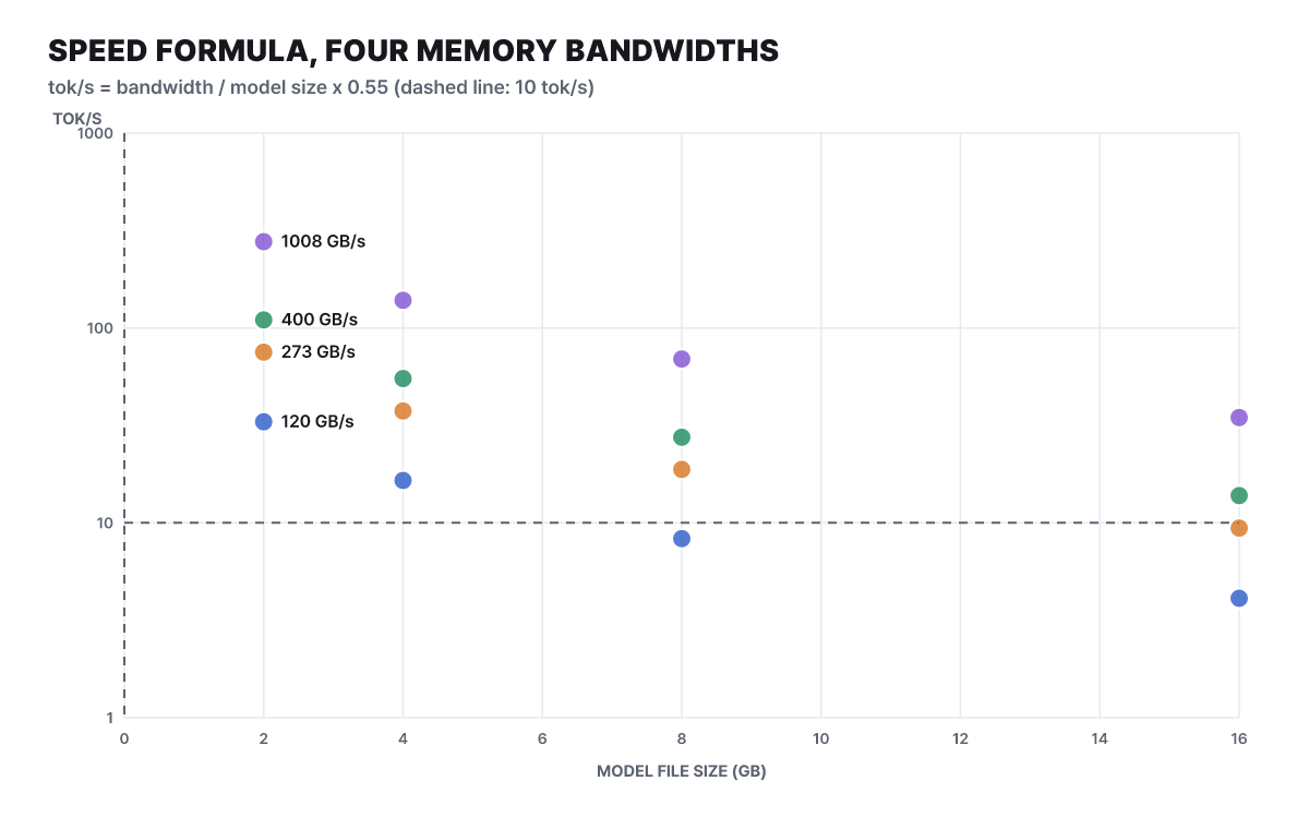Figure 3. Results of the speed formula (editors’ calculation, the four bandwidths are assumed, efficiency factor 0.55)

At 120GB/s of bandwidth, the same model gets about 16 tokens at 4GB, about 8 tokens at 8GB and about 4 tokens at 16GB. Double the model size and the speed is exactly halved. The 7B Q8_0 in Figure 1 (assumed 7.5GB) landing around 9 tokens at 120GB/s also comes from this formula. Conversely, at a high bandwidth such as 1008GB/s, even a 16GB model sits above the dotted line. So two models with the same rank can be awkward to use on a laptop and comfortable on a desktop GPU, which is why you should read the tok/s column alongside the ranking, not the ranking alone.

For GPUs missing from the table, the fallback formula K ÷ parameters (B) × quantization multiplier uses a backend constant. The constants are CUDA 220, Metal 160, ROCm 180, SYCL 100, ARM CPU 90, x86 CPU 70 and Ascend NPU 390. If you know a card’s bandwidth, you can write it in yourself with gpu_bandwidth_gbps_override, and you can check which value was used by going back through estimate_basis.

Time to first token (TTFT) and prompt processing speed are different calculations. Reading the prompt is limited by compute, not bandwidth, so llmfit gives a value only when it knows the GPU’s fp16 compute performance, and when it does not, it leaves the value empty (null) rather than 0. Writing 0 would read as “too slow to measure.”

Conf on every cell, the trust ladder

llmfit attaches a trust level to each speed estimate. The priority order, which the docs say “the first match wins,” is as follows.

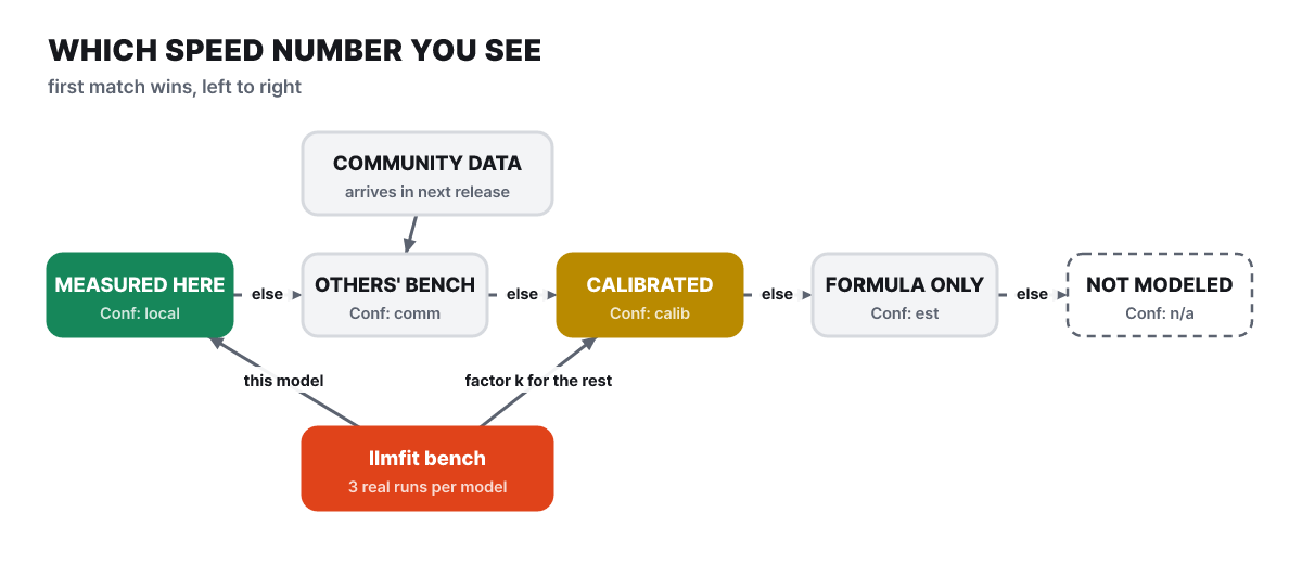Figure 4. At which level a number in the speed column gets adopted

The further left in the figure, the more trustworthy. local is a value you measured on your own computer with llmfit bench, comm is a value another user measured on the same hardware, calib is the formula multiplied by a calibration factor obtained from measurements on this hardware, and est is the formula alone with no measurement. n/a is the case where the model needs a runtime llmfit cannot model, so there is no estimate at all.

The arrow at the bottom is the most interesting part of this structure. According to the docs, a measurement from a dense model of 1B or more is used as a factor that calibrates the estimates for every other model on the same hardware, and the detail screen shows it in the form “Calibrated ×N.” Records measured on a different CPU or GPU configuration are ignored. In effect, measuring just one model turns the est across the whole list into calib. When the same number exists in several places, the priority is the value you measured yourself, the community value for the same hardware, the median from a public benchmark database (localmaxxing), and then the formula estimate.

The community values at the top are the route by which merged pull requests ride along into the next release. The repository history shows that on Oct 26 alone, community benchmark data for several pieces of hardware, such as Apple M5 Pro, GeForce RTX 5060 Ti and Radeon RX 7900 XT, was merged. That data is a change after v1.1.17, so it goes into the next release. If your hardware is on the list, est may have turned into comm after you upgrade.

Measure it yourself to turn est into local

If the speed estimate bothers you, measure it. llmfit bench sends three actual inference requests to a running runtime (Ollama, vLLM, LM Studio, MLX, llama-server and so on) and measures tokens per second and time to first token. For the laptop example, download the model you chose in step 4, bring it up in a runtime, and proceed as follows.

1. In the TUI, bring up the model you downloaded with d in a runtime and refresh the installed list with r. Installed models are marked in the Inst column
2. To measure a single model, specify the provider and model, as in llmfit bench --provider ollama llama3.2. --all measures every model it finds, and --quality --routing gives per-role quality scores and a routing table
3. The result is saved first on your own computer (the bench store in ~/.config/llmfit). It does not disappear if you do not share it, and it replaces the list's estimates with local values
4. Sharing is optional. With llmfit bench --all --share, it forks the GitHub repository, uploads a result file under llmfit-core/data/community/<hardware>/ and opens a pull request

The sharing step needs GitHub authentication. According to the docs, the gh command is not required; it uses either device authentication, where you approve a code once in the browser, or the GITHUB_TOKEN environment variable. Nothing is uploaded until you agree in the confirmation window, and adding --dry-run previews the JSON that would be uploaded without using the network. Merged results ride in the next release and show up as measured values (✓) in the tables of users with the same CPU and GPU combination. This article explains things from the CLI, and you can check the keys used inside the TUI in the h help.

Ask before you buy: profiles, plan, storage

Go one step further from the laptop example and you end up asking, “what computer would I need to buy to run this model?” llmfit can run the same calculation on a computer that is not yours. The ways to change capacity only are --memory (VRAM), --ram, --cpu-cores and the percent option seen earlier. To change bandwidth too, use a hardware profile (--profile). The bundled profiles the docs introduce include nvidia-rtx-4090, apple-m3-max-128gb and ryzen-ai-max-plus-395.

llmfit hardware list                                    # bundled and user profiles
llmfit --profile nvidia-rtx-4090 recommend --json       # if you had this card
llmfit --profile ryzen-ai-max-plus-395 plan "openai/gpt-oss-120b" --context 8192 --target-tps 25

A profile is a small JSON file. The fields the docs define are schema_version (1), name (must match the file name), match.gpu_name_contains, hardware.total_ram_gb, hardware.unified_memory, hardware.gpu_memory_bandwidth_gbps and hardware.ddr_bandwidth_gbps, and hardware.gpu_compute_tflops_fp16 is optional. Leave it out and the TTFT side stays null, not 0. Below is an example filled with assumed values.

{
  "schema_version": 1,
  "name": "my-workstation",
  "hardware": {
    "total_ram_gb": 64,
    "unified_memory": false,
    "gpu_memory_bandwidth_gbps": 900,
    "ddr_bandwidth_gbps": 80
  }
}

After saving, checking with llmfit hardware validate ./my-workstation.json catches key typos. The failure output the docs show looks like this.

FAIL  ./my-workstation.json: unknown key(s): hardware.gpu_bandwith_gbps

The reason to write the bandwidth is that the speed estimate is computed from that value. --memory, which changes capacity only, answers just “which models fit” and uses the host’s own bandwidth for “how fast.” --profile cannot be combined with --memory, --ram or --cpu-cores, and it cannot yet be combined with --force-runtime either.

plan flips the direction and starts from the model. Give llmfit plan "<model>" --context N [--quant Q] [--target-tps N] a context length and a target speed, and it calculates the minimum and recommended hardware, and whether each path, GPU, CPU offload or CPU-only, is feasible. If you will download several models and swap between them, you have to count the SSD as well. The defaults of llmfit storage are 3 models, a 100GB OS reserve, scratch space for the one largest model, and 15% headroom to leave. The docs’ formula is as follows.

need_gb            = os_reserve_gb + library_gb + download_scratch_gb
target_capacity_gb = need_gb / (1 - headroom_percent / 100)

The minimum SSD is need_gb, and the recommended SSD is target_capacity_gb, each rounded up to the first value above it in the tier list (256, 512, 1000, 2000, 4000, 8000, 16000, in decimal GB). If three models total 60GB and the largest is 25GB, the required capacity is 100 + 60 + 25 = 185GB and the recommended calculation is 185 ÷ 0.85 ≈ 218GB, so both land in the 256GB tier. The docs state the limits too. It counts weights only (all experts for MoE), it does not scan free disk space, it does not cover running several models at once, and the reserve and headroom values are planning values you adjust, not measurements.

How scripts and agents call the same calculation

There are three ways to get the same verdicts without going through the screen. The first is JSON output.

llmfit recommend --json --use-case coding --limit 3   # top 3 for coding, as JSON
llmfit fit --perfect -n 5                              # only 5 Perfect verdicts
llmfit info "Mistral-7B"                               # fit analysis and the basis of estimates for one model

The second is REST. You open it with llmfit serve, and the key endpoint is /api/v1/models/top, which asks for the top models a single node can run right now. There are also /api/v1/system, /api/v1/concurrency for concurrent-session capacity and /api/v1/storage for the SSD calculation, and when only the same computer uses it, you can open it over a Unix socket (--unix-socket) instead of a network port. Concurrent sessions have also been calculated by llmfit concurrency <model> --json since v1.1.16. It shows how many sessions fit for each context between 4,000 and 256,000 tokens, and the differences by KV cache precision (fp16, fp8, q8_0, q4_0). As the docs make clear, this is a ceiling on how many fit in memory, not throughput under load.

The third is MCP. llmfit serve --mcp exposes six tools over standard input and output.

MCP tool	What it does
get_system_specs	RAM, GPU and CPU information
recommend_models	Top models filtered by use case, minimum fit, runtime and license
search_models	Text search by name and provider
plan_hardware	Hardware needed for a model, context, quantization and target speed
get_runtimes	Installed inference runtimes
get_installed_models	Models present in local runtimes

The repository also includes a skill for OpenClaw agents (skills/llmfit-advisor). Once installed, the agent reads the specs with llmfit --json system, gets a ranking with llmfit recommend --json, maps Hugging Face model names to Ollama, vLLM and LM Studio tags, and asks the user whether to update the Ollama model list in openclaw.json.

Runtime integrations switch on automatically for whichever is detected. For Ollama, if a daemon is running at localhost:11434, it reads the installed model list (/api/tags), puts a check mark in the table’s Inst column, and downloads the model when you press d. To point at Ollama on another computer, use OLLAMA_HOST. A setup that runs llmfit on the laptop and reads the Ollama on a GPU server is also possible. llama.cpp is found as an executable on PATH (set the location with LLAMA_CPP_PATH) and downloads GGUF files directly, while Docker Model Runner defaults to localhost:12434 and LM Studio to 127.0.0.1:1234.

Where you get stuck, and the order with llm-checker

The places people usually get stuck while following along are these five.

• Environments where detection fails: According to the docs, Windows is detected from RAM, CPU and an NVIDIA GPU with nvidia-smi, and on Android (Termux and so on) the GPU cannot be detected. In that case you can still get recommendations by writing it in yourself, as in --memory=8G
• The catalog is built in: The model list is inside the binary, so new models arrive when you upgrade. If you do not want to wait, llmfit update fetches popular models from Hugging Face, or you can write your own entries in the custom model file custom_models.json with name, provider, parameter count, minimum and recommended memory, quantization, context length and use case. With the same name, your entry wins
• The quality score is simplified: It relies on family reputation and a table compiled from public leaderboards, so it does not guarantee performance on your own work
• Speed is a formula value: While Conf is est, tok/s can differ from reality depending on context length and runtime
• Windows installer signing varies by release: According to the README, only releases whose signing job succeeded to the end are signed, so check the signature if you need it

This tool moves fast. In the month from v1.1.15 (Sep 10) to v1.1.17 (Oct 8), it gained concurrent-session estimates, disk planning, 1.58-bit model recognition, the percent option, mouse support and rank pinning, and after the release, on Oct 25 and 26, a multi-word search fix, an F32 model scoring fix and a change allowing sizing flags after a subcommand landed on main. These changes are not yet in a release. The README also introduces a sister project, llmfit-gui, a desktop GUI for Windows.

The alternative the README introduces is llm-checker. It is a Node.js tool that differs in that it actually downloads and runs models through Ollama, and the docs note that it does not distinguish MoE structures and treats everything as a dense model. The two tools are less competitors than different steps in an order. To narrow candidates before downloading, llmfit fits, and to run and verify after you have narrowed them, llm-checker fits. llmfit’s bench also covers the step that corresponds to that “run it and see.”

Back to the scene at the laptop: the ranking this tool gives is less an answer than a hypothesis produced by that day’s catalog and formulas. That the same laptop can show a different ranking and different Conf cells after one upgrade actually speaks to its usefulness. The hypothesis comes with a way to refute it, the refutation is one command (llmfit bench), and one refutation fixes the numbers across the whole list. It is a structure in which you end up with a far more trustworthy table after running bench once than when you first opened the ranking.